VLOOKUP Formula to Compare Two Columns in Different Excel Sheets |
您所在的位置:网站首页 › compare two excel sheets for differences › VLOOKUP Formula to Compare Two Columns in Different Excel Sheets |
VLOOKUP Formula to Compare Two Columns in Different Excel Sheets
|
Get FREE Advanced Excel Exercises with Solutions!
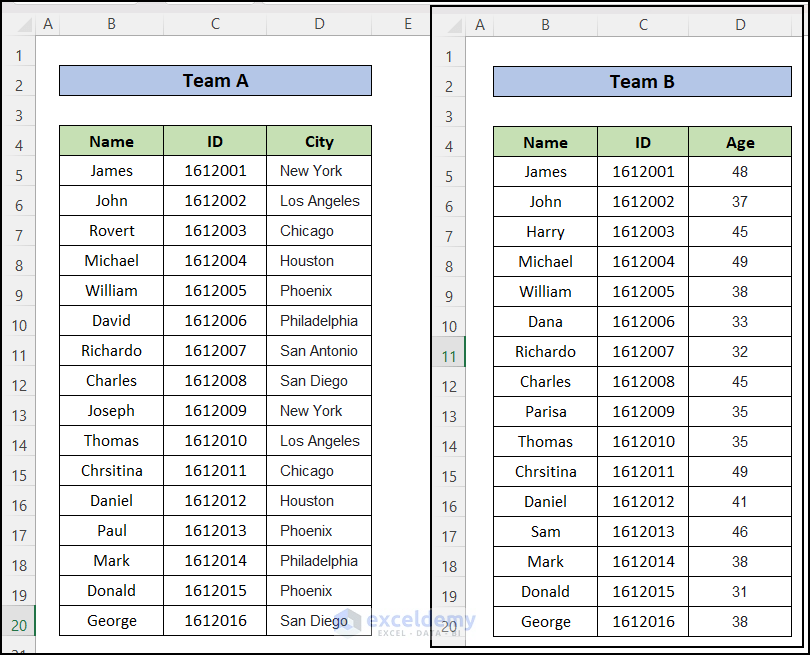
If you are searching for some special tricks to use the VLOOKUP Formula to compare two columns in different sheets then you have landed in the right place. There are some easy ways to use the VLOOKUP formula to compare two columns in different Sheets. This article will show you each and every step with proper illustrations so, you can easily apply them for your purpose. Let’s get into the central part of the article. Table of Contents hide Download Practice Workbook 3 Examples Using VLOOKUP Formula to Compare Two Columns in Different Excel Sheets 1. Compare Two Columns in Different Excel Sheets and Return Common/ Matched Values 2. Compare Two Columns in Different Worksheets and Find Missing Values 2.1 Using Filter Feature 2.2 Using FILTER with VLOOKUP Function 3. Compare Two Lists in Different Worksheets and Return a Value from a Third Column VLOOKUP for Multiple Columns in Different Sheets in Excel with One Return Only Conclusion Related Articles Download Practice WorkbookYou can download the practice workbook from here: Compare Two Columns in Different Sheets.xlsx 3 Examples Using VLOOKUP Formula to Compare Two Columns in Different Excel SheetsIn this section, I will show you 3 quick and easy methods to use the VLOOKUP Formula to compare two columns in different sheets on Windows operating system. You will find detailed explanations with clear illustrations of each thing in this article. I have used Microsoft 365 version here. But you can use any other versions as of your availability. If anything of this article doesn’t work in your version then leave us a comment. Here, I have data from two teams that have some common members in two different worksheets named “TeamA” and “TeamB”. And, I will show you how you can find the common names and the different names of the two teams.
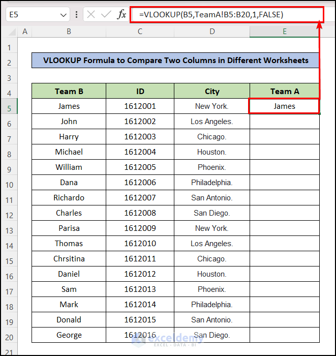
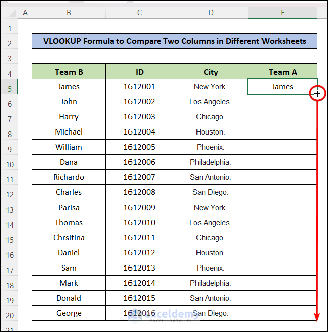
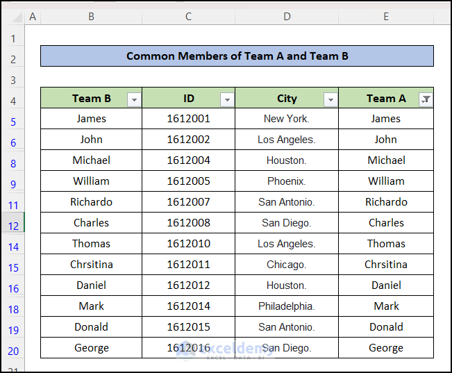
First, I will show you how to use the VLOOKUP function to find common names or the matched values of two different lists of names in different worksheets. Follow the steps below for this: Here, I will try to get the common names of Team A and Team B. For this, I have created a new worksheet that already contains the data of Team B. Then, I created a new column to find the common names. Then, insert the following formula into cell E5: =VLOOKUP(B5,TeamA!B5:B20,1,FALSE)
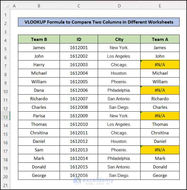
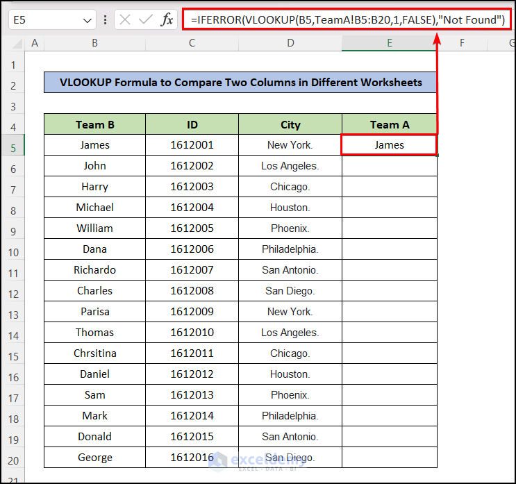
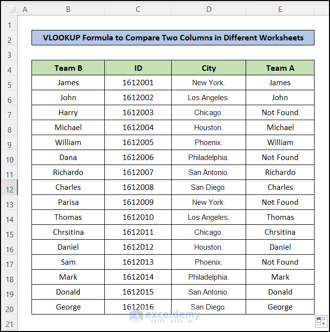
Read More: How to Use VLOOKUP Function to Compare Two Lists in Excel Using IFERROR with VLOOKUP Function to Treat the #N/A Error: To avoid the showing of ‘#N/A Error” in the column, you can use the IFERROR function with the VLOOKUP function. For this, insert the following formula into cell E5: =IFERROR(VLOOKUP(B5,TeamA!B5:B20,1,FALSE),"Not Found")🔎 Formula Breakdown: To understand this formula, you must be familiarized with the IFERROR excel function. The syntax of IFERROR function: =IFERROR(value, value_if_error) Let’s see how the above formula works As the value of IFERROR function, we have input our VLOOKUP So, if there is no error, the output of the VLOOKUP formula will be the output of the IFERROR function. As the value_if_error argument, we have passed this value, “Not Found”. So, if IFERROR function finds an error in the cell, it will output this text, “Not Found”.
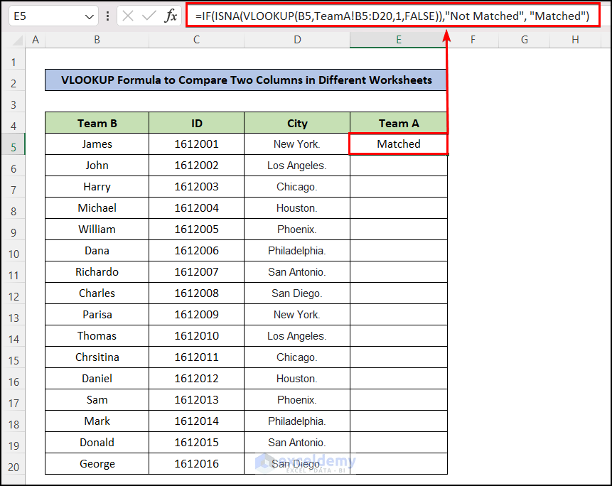
Using IF and ISNA with VLOOKUP Function to Handle the #N/A Error: There is another way to find avoid the #N/A Error and that is using IF and ISNA functions with VLOOKUP functions. For this, paste the following formula into cell E5: =IF(ISNA(VLOOKUP(B5,TeamA!B5:D20,1,FALSE)),"Not Matched", "Matched")
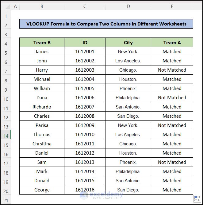
🔎 Formula Breakdown: Let’s now see how the following formula works. As the logical_test argument of the IF function, we have passed the ISNA function and the ISNA function holds our VLOOKUP If the VLOOKUP formula returns a #N/A error, the ISNA function will return the TRUE When the logical_test is true IF function will return this value: “Not Matched”. If the VLOOKUP formula returns a value (no error), the ISNA function will return FALSE So, IF function’s logical_test argument will be False. When logical_test is False IF function will return this value: “Matched”. Thus, you will get the column filled with “Matched” and “Not Matched” values. Now you can easily identify the common names between the name lists of separate worksheets.
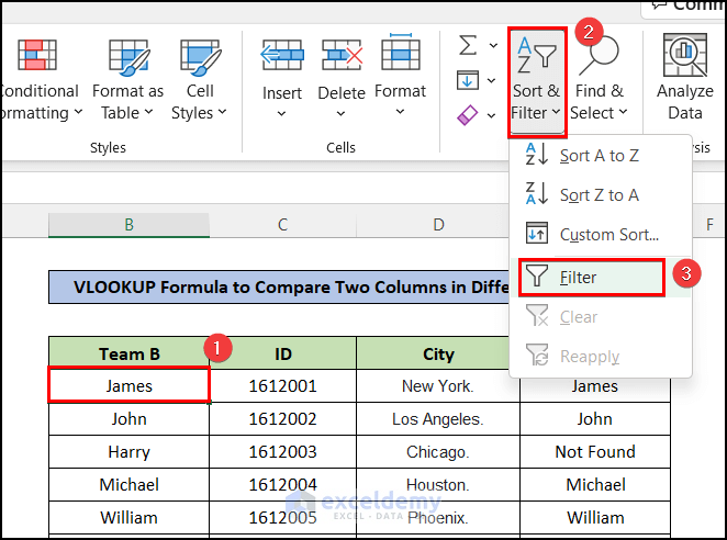
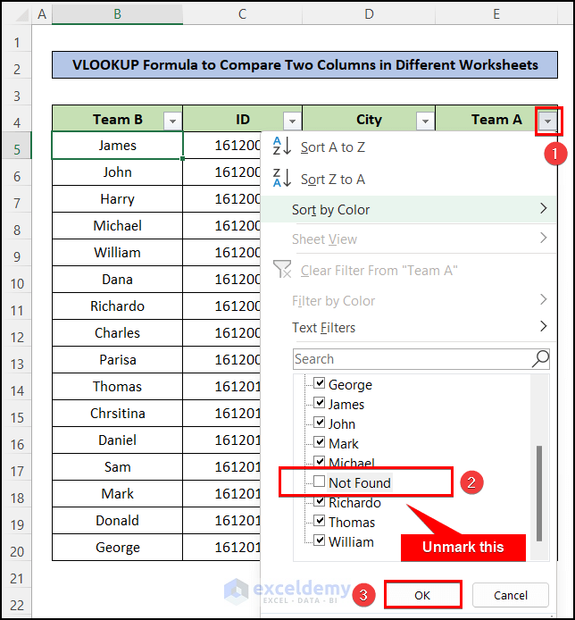
Read More: Excel Formula to Compare and Return Value from Two Columns Similar Readings How to Compare Text of Two Cells in Excel (10 Methods) Excel Compare Text in Two Columns (7 Fruitful Ways) How to Count Matches in Two Columns in Excel (5 Easy Ways) Excel formula to compare two columns and return a value (5 examples) How to Compare Two Columns for Finding Differences in Excel 2. Compare Two Columns in Different Worksheets and Find Missing ValuesIn the previous example, you have got how to find the common names of two different lists in different worksheets, Now, I will show you how you can find the missing values of a list compared to another list. 2.1 Using Filter FeatureSimilarly, before, you can use the Filter feature to find the missing values. After using the VLOOKUP with the IFERROR function, you have already a column that is showing “Not Found” values for the mismatched names. Now, go to the Filter option again by clicking the Filter arrow in the column header of “Team A”. Then, unmark all the checkboxes except that saying “Not Found”. Then, press OK. |
【本文地址】